https://arxiv.org/pdf/2411.03312
https://github.com/locuslab/llava-token-compression.
Let me format the text with line breaks for each sentence:
Vision Language Models (VLMs) have demonstrated strong capabilities across various visual understanding and reasoning tasks.
However, their real-world deployment is often constrained by high latency during inference due to substantial compute required to process the large number of input tokens (predominantly from the image) by the LLM.
To reduce inference costs, one can either downsize the LLM or reduce the number of input image-tokens, the latter of which has been the focus of many recent works around token compression.
However, it is unclear what the optimal trade-off is, as both the factors directly affect the VLM performance.
We first characterize this optimal trade-off between the number of visual tokens and LLM parameters by establishing scaling laws that capture variations in performance with these two factors.
Our results reveal a surprising trend: for visual reasoning tasks, the inference-optimal behavior in VLMs, i.e., minimum downstream error at any given fixed inference compute, is achieved when using the largest LLM that fits within the inference budget while minimizing visual token count — often to a single token.
While the token reduction literature has mainly focused on maintaining base model performance by modestly reducing the token count (e.g., 5 – 10×), our results indicate that the computeoptimal inference regime requires operating under even higher token compression ratios.
Based on these insights, we take some initial steps towards building approaches tailored for high token compression settings.
3.1 SCALING LAW FORMULATION
Recall that the performance of a VLM is primarily governed by the parameter count of the language model and the number of visual tokens processed by the LLM, assuming a fixed visual encoder.
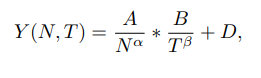
Accordingly, we model the scaling behavior of VLM performance as:
Let me help format the long text with line breaks for each sentence:
where N denotes the LLM parameters, T denotes the input visual tokens, {A, B, D, α, β} are learnable parameters, and Y (N, T) is a measure of model quality.
Although traditional scaling laws have been studied in the context of pretraining loss Kaplan et al. (2020), practitioners often use the direct downstream performance to assess model quality (Gadre et al., 2024; Goyal et al., 2024b; Liu et al., 2022).
Thus, we use average downstream error on a suite of nine commonly used visual reasoning benchmarks (§ 3.2) as a measure of model quality Y (N, T).
Below, we summarize the role of each of these learnable parameter in the scaling law (Eq. 2).
LLM Quality Parameter (α): This parameter dictates how the downstream error changes with the complexity of the LLM, i.e., its parameter count.
A larger α indicates a better language model, such as Llama3-7B outperforming Llama2-7B, which often stems from better pretraining.
Visual Token Quality Parameter (β): β captures the quality of the visual input tokens fed into the LLM, reflecting the quality of the compression technique.
A more effective token compression algorithm would yield a larger β, allowing for more reductions in number of T visual tokens than less effective methods while maintaining the same downstream performance.
Constants (A, B, D): A and B are normalizing constants and D refers to irreducible loss, which cannot be reduced even with the largest N-sized language model or all T visual tokens (capped at 576 for our choice of vision encoder).
3.2 EXPERIMENTAL SETUP
VLM Training and Evaluation: We use the LLaVA-Next framework (Liu et al., 2024b) to train VLMs with the Qwen-1.5 family of language models as the backbone.
Specifically, we utilize the Qwen-{0.5, 1.8, 4, 7, 14}B-chat models (Bai et al., 2023).
The pretraining and finetuning dataset and hyperparameters follow Liu et al. (2024a), except we double the effective batch size for finetuning.
We use CLIP ViT-L/14 (Radford et al., 2021) as the vision encoder for all experiments, and compress the original 576 tokens to {144, 64, 36, 16, 4, 1} tokens using TokenPacker (Li et al., 2024c).
To estimate the downstream error Y (N, T), we evaluate on 9 commonly used benchmarks for visual reasoning and understanding: MME (Fu et al., 2024), GQA (Hudson & Manning, 2019), AI2D (Kembhavi et al., 2016), MMBench (Liu et al., 2024c), MMMU (Yue et al., 2023), ScienceQA (Lu et al., 2022), MathVista (Lu et al., 2024), POPE (Li et al., 2023c), and ChartQA (Masry et al., 2022).
We compute Y (N, T) by averaging the errors of the normalized evaluation metric.
For MME, the Cognition and Perception scores were combined and the F1 scores were used for POPE.
Fitting Scaling Laws: We fit the proposed scaling law (Eq. 2) on {Y (N, T), N, T} pairs, with N ∈ {0.5B, 1.8B, 4B, 7B} and T ∈ {1, 4, 16, 36, 64, 144, 576} (described in the experiment setup above).
We use grid-search, for its stability (Goyal et al., 2024b), to estimate the scaling parameters α, β, A, B, and D.
The final scaling law is evaluated on a N = 14B VLM model at various number of visual tokens in T.
Further details about the grid-search fit can be found in Appendix A.2.
3.3 RESULTS: ESTIMATED SCALING CURVES
Recall from Section 2.1 that F LOP sinf = O(N(Q+V )), where Q represents the input text tokens, and V is the visual input tokens.
We first visualize our scaling laws under 2 settings — (a) cached text input (Fig.1a): The input text tokens (Q) are fixed and can be cached, leading to F LOP sinf ∼ O(NV ), and (b) non-cached text input (Fig.1b): The input text tokens are approximated as 50, i.e., F LOP sinf = O(N(50 + V )) (we consider more granular variation of Q in § 3.3.2).
Figure 1 visualizes the fitted scaling curve, illustrating the variation in the average downstream error as inference FLOPs are varied (under both the cached and non-cached text input setting).
We vary the inference FLOPs on the x-axis by increasing the number of visual input tokens processed by the LLM (the scatter size), while the color scale indicates the varying number of language model parameters.
We make some key observations below.
Log Linear Relation between Error and Number of Visual Input Tokens: Consider the change in performance for the 7B model as the number of visual input tokens varies (maroon curves in Fig. 1.)
Recent works on visual token compression (Li et al., 2024c; Shang et al., 2024) claim little to no performance degradation with token compression.
For example, they report similar performance to the base model's 576 tokens even when visual token count is reduced to 36 or 144 on certain tasks.
However, our scaling curves in Figure 1a reveal a different trend, showing a log-linear decrease in visual reasoning performance as the number of visual input tokens is reduced.
We believe this discrepancy arises because of the limited downstream evaluation benchmarks considered in the previous works which may not fully capture the VLM's overall capabilities.
Error Varies 5× Faster with LLM Parameters than with Tokens: Recall from the scaling law (Eq. 2) that α represents the LLM quality parameter and β represents the visual token quality parameter, both denoting the rate at which they influence the downstream error respectively.
From Figure 1a, we observe that α = 0.077 is more than five times larger than β = 0.015, signifying that VLM error increases significantly faster when reducing the LLM parameters compared to reducing the number of visual tokens.
Therefore, when minimizing inference FLOPs, it is more effective to prioritize reducing visual tokens (V ) first, as the impact on performance is less pronounced than reducing the LLM parameters (N).
This finding is reflected in Figure 4 where we observe that, under fixed inference compute, using a larger LLM with fewer visual tokens (7B LM w/ 36 tokens) provides better performance than using a smaller LLM with more visual input tokens (1.8B LM w/ 144 tokens) for visual reasoning tasks.
Scaling Laws Hold for Increases in LLM Scale:
We evaluate the accuracy of our scaling laws (fitted on VLMs of 0.5B-7B range) for predicting the performance for larger models.
We estimate the performance of Qwen-1.5 14B using our fitted scaling laws.
Our scaling laws estimate the performance with an error margin of less than 2%, as visualized in Figure 2, 6b.
The log-linear relationship between the error and number of visual tokens persists, and the greater influence of the LLM’s size compared to visual tokens on performance continues to hold.
Thus, for VLMs using 7B language model backbones, it is still optimal to increase LLM size to 14B while reducing visual token count for fixed inference costs

3.3.1 COMPUTE-OPTIMAL INFERENCE REQUIRES A SINGLE VISUAL TOKEN
Observe the pareto optimal curve (black dotted curve) in Figure 1a.
For cached query, at any given inference compute, the optimal behavior, i.e., lowest downstream error, occurs when using the largest possible LLM while reducing the number of visual input tokens to one.
Thus, for scenarios where the text input can be cached (Q = 0), such as monitoring systems with static text input, one should utilize the largest LLM possible by reducing the number of visual tokens to fit the inference budget.
A similar trend of prioritizing the LLM size holds in the variable text input regime.
For example, in Figure 1b, where the text input length Q = 50, better performance in a fixed compute budget often results from the larger model with fewer visual tokens with the optimal number of visual tokens is now around 16 (intersection of pareto curve with scaling plot).
This increase in optimal visual tokens as text tokens increase is intuitive, as the VLM incurs a fixed cost for processing the text.
Thus, small increases in the number of visual tokens lead to only minor increases in the overall inference cost while improving performance.
The key observation is that compute-optimal behavior entails using the largest feasible LLM with very few visual input tokens.
This result has important consequences.
Existing literature on token reduction (§ 5) has primarily focused on moderately reducing the number of visual input tokens (e.g., from 576 tokens to 144 or 64 tokens) while trying to match the performance of the base model.
However, our results highlight that it is better to operate in a regime with much lower input visual tokens (e.g., 1, 4 or 16), as exchanging visual tokens for larger LLM size reduces the downstream error.
This highlights the need to develop token compression techniques tailored for extreme token compression.
We take some initial steps in this direction, building on existing token compression algorithms in Section 4.
3.3.2 VARIATION IN OPTIMAL TOKENS WITH TEXT QUERY LENGTH
The shift in performance trends and the ideal visual token count from Q = 0 → 50 raises the question; how does the input text length impact the optimal selection of LLM size and number of visual tokens?
To explore the variations in trends, we consider the effect of text input length on the optimal inference behavior in Figure 3a.
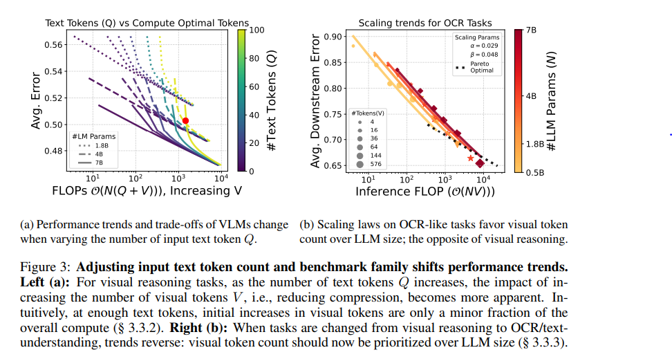
First, when the text input length, Q, is small (purple curves), it is always better to use the larger model (solid curve) with less visual tokens compared to the smaller model (dashed curve) with more visual tokens.
However, consider an edge case where the text input length is extremely high (e.g., 100 for the green curves).
We observe that there is a sharp increase in error as inference FLOPs are reduced.
This is because visual tokens need to be reduced significantly for any effective change in inference FLOPs, as the fixed cost from text tokens is quite high.
At a certain point (marked by the red dot in Figure 3a), it becomes more advantageous to use the 4B model with a higher number of visual tokens rather than the 7B model with fewer tokens (contrary to the case for lower Q).
Thus, the optimal number of visual input tokens rises with an increase in Q.
This case demonstrates the need for careful balancing of visual token count and LLM size, especially in scenarios where text inputs are long, to achieve compute-optimal performance without sacrificing accuracy.
Despite the changes in the exact optimal visual token count and LLM parameter count as the length of the user query increases, the general trend for visual reasoning and understanding tasks is that increasing the size of the language model while reducing visual tokens can lead to significant relative gains (as also illustrated in Fig. 4).
This finding may be due, in part, to the scaling properties of the LLMs, which allow larger models to extrapolate with less visual information than their smaller counterparts (Radford et al., 2021; Wei et al., 2022).
However, this trade-off does not extend to certain tasks, such as document comprehension, text identification, etc., where a single or handful of tokens may not be able to incorporate the high density of information, and the trend starts to reverse, as we discuss in detail in § 3.3.3.
Scaling Inference Compute by Simply Repeating Tokens: Many recent works around scaling test-time compute by introducing special tokens (Goyal et al., 2024a) or multiple parallel generations (Zelikman et al., 2024) have shown promising gains in reasoning tasks for language models.
We test this notion with VLMs by repeating the visual input tokens (compressed to 4) multiple times to allow for more processing of key visual aspects.
However, we do not observe any performance gains.
This is most likely due to the fact that the downstream tasks for VLMs are not as reasoningintensive, which demonstrates the importance of developing better token compression algorithms and potentially introducing more challenging benchmarks.
3.3.3 SCALING LAWS FOR OCR TASKS
Until now, we have focused on scaling behavior for visual reasoning and understanding tasks, highlighting the key finding that using a single visual token with the maximum possible LLM parameters is the inference-optimal configuration.
However, is the same valid for all tasks?
VLMs have recently been applied to document reading and OCR-style tasks where a single visual token may be insufficient due to the high density of information.
Unlike visual reasoning tasks, these tasks lack visual structure in the image and intuitively need more tokens to record the (generally textual) details in the image.
We verify the same by fitting our scaling laws (Eq. 2) on DocVQA (Mathew et al., 2021) and TextVQA (Singh et al., 2019) benchmarks, where the tasks require mainly OCR capabilities.
Figure 3b presents the fitted scaling law for OCR tasks.
Notably, there are no significant gains in average downstream performance from increasing LLM parameters; instead, the number of visual tokens predominantly dictates the performance.
This observation is reflected in the scaling law parameters, where the LLM-quality parameter α = 0.029 is nearly twice as smaller than the token quality parameter β = 0.048.
This trend is in stark contrast to the scaling parameters observed for visual reasoning tasks where the LLM-quality parameter (α) was more than five times larger than the token parameter (Fig. 1a).
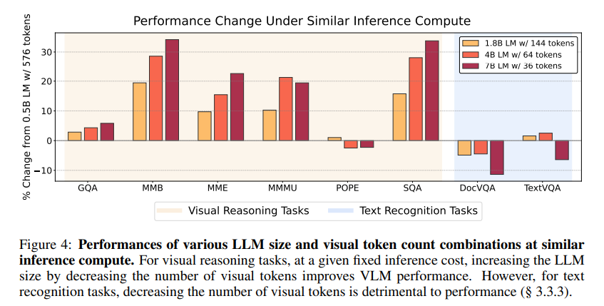
This notion of visual tokens playing the significant role in OCR tasks is further echoed in Figure 4, which shows token compression weakens VLM performance despite increasing the size and capabilities of the LLM component to compensate.
the token parameter (Fig. 1a).
This notion of visual tokens playing the significant role in OCR tasks is further echoed in Figure 4, which shows token compression weakens VLM performance despite increasing the size and capabilities of the LLM component to compensate.
4 QUERY-BASED TOKEN COMPRESSION
The Need for Token Compression in Extreme Regimes: While prior work has primarily focused on moderately compressing the tokens (e.g., reducing 576 tokens to 144) while trying to match the performance of the base model (no token compression), our findings (§ 3.3.1) suggest the need for a paradigm shift.
Rather than aiming for moderate token compression, new approaches should be tailored for extreme token reduction — down to 1, 4, or 16 tokens — with minimal possible degradation, as our scaling laws demonstrate that compute-optimal behavior is within this range.
Our work takes initial steps in this direction by introducing a query-based token compression strategy designed for such high-compression regimes.
In cases where tokens are reduced to as few as 1, token compression based on the user's input query becomes critical for retaining relevant information and minimizing performance reductions.
In the following section, we build on existing algorithms (Li et al., 2024c), to incorporate query-based token compression.
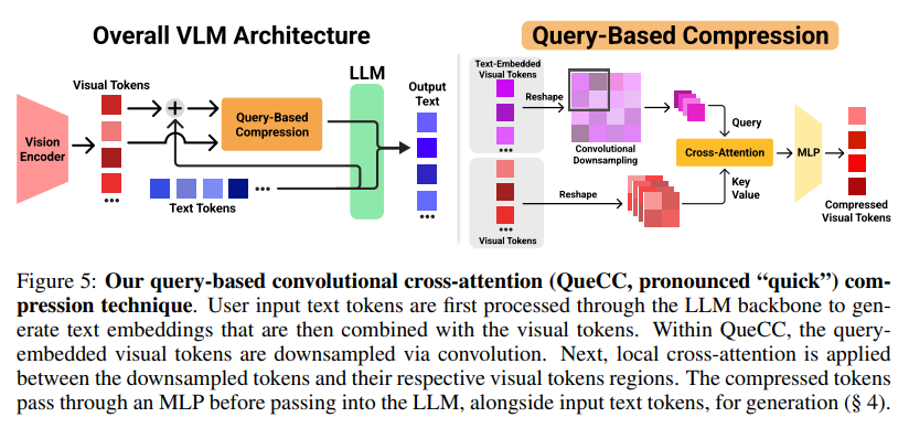
Figure 5 summarizes our query-based convolutional cross-attention (QueCC, pronounced "quick") compression technique.
User Query Information Injection: To make our projector query-dependent, we add the text embedding of the user's most recent query to the image embeddings from the vision encoder.
We do this by taking the last hidden states prior to the LM head of the user input from the language model as the representation of the user's overall query.
The hidden state is converted into the text embedding via a linear projection and added to the image visual token embeddings.
These fused tokens are later used as the query component for cross-attention.
The text embedding can easily be cached for applications where the query is static or is part of a predetermined set.
Even if the query varies, the text-embedding can be precalculated prior to processing the image and KV values cached and reused when processing the visual and text tokens together during generation.
Token Downsampling with Cross-Attention and Learnable Convolutions: To compress the number of visual tokens passed into the LLM, we utilize a region-based, cross-attention mechanism that downsamples the vision encoder tokens, X, into a more information-dense form.
The mechanism hinges on viewing X as a √ n × √ n grid due to the patchification of the image by the vision encoder.
Li et al. (2024c;d) passes the "2D" version of X through a downsampling function that compresses the input by a s 2 factor where each resulting token corresponds to a s × s region in the original input.
After this, cross-attention is applied independently between each downsampled token and the corresponding tokens in its s × s region.
We improve on the bilinear interpolation-based downsampling techniques (Li et al., 2024c; Wang et al., 2024b) by using a learnable, depth-wise 2D convolution filter of kernel size and stride s, providing better expressivity.
4.1 EXPERIMENTAL SETUP
We use a training setup similar to LLaVa-1.5 (Liu et al., 2024a) and use Vicuna-1.5 7B as the LLM.
Based on the optimality of high token compression underscored by our scaling laws (§ 3.3), we focus on visual token budgets of {1, 4, 16, 36, 64}, corresponding to compression rates of 88.9% to 99.8%.
We benchmark our method on a diverse, comprehensive set of visual reasoning/understanding and OCR/text-understanding tasks: GQA (Hudson & Manning, 2019), MMBench (MMB) (Liu et al., 2024c), MME (Fu et al., 2024), POPE (Li et al., 2023c), ScienceQA (SQA) (Lu et al., 2022), TextVQA (Singh et al., 2019) VizWiz (Gurari et al., 2018), and VQAv2 (Goyal et al., 2017).
4.2 QUERY-BASED CONVOLUTIONAL CROSS-ATTENTION (QUECC) RESULTS
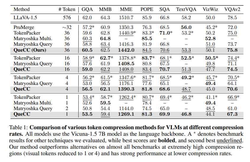
Table 1 presents the results of our QueCC algorithm in comparison to previous methods, including TokenPacker (Li et al., 2024c), LLaVa-PruMerge (Shang et al., 2024), Matryoshka Multimodal Models (Cai et al., 2024), and Matryoshka Query Transformer (Hu et al., 2024), in low token regimes.
We find that our method performs better than alternatives at the highest compression levels in multiple different data sets, leading to a 12% and 19% improvement in the gap between the original LLaVA-1.5 model and the next-best method on MME and MMB for the one-visual-token level.
The trend continues at the four-token level, where the gap between QueCC and the next-best algorithm was reduced by 26% and 21% on MME and MMB.
Our model exhibits strong performance on GQA, MME, SQA, and VQAv2 across compression rates, signaling the prospects of using the user's query to identify and compress key visual tokens.
5.2 SCALING LAWS AND SCALING INFERENCE COMPUTE
Understanding how the performance of modern deep networks improves as key design factors, such as the number of parameters or training tokens, are scaled has become a focal point of research, particularly as these models continue to grow in size and complexity.
Scaling laws offer crucial guidance for optimizing the architecture of such models.
Notably, Kaplan et al. (2020); Hernandez et al. (2021); Hoffmann et al. (2022) do a thorough investigation into training compute-optimal language models, highlighting the need to scale pretraining tokens and parameters at the same rate.
Cherti et al. (2023); Gadre et al. (2023) perform a similar study on scaling laws for CLIP (Radford et al., 2021), corroborating that performance improvements arise from increasing both parameter counts and pretraining image-caption pairs.
Closest to our work, Li et al. (2024a) investigate what factors improve the performance of LLaVA (Liu et al., 2023).
They observe performance gains with increasing language model size, visual encoder size, and input resolution.
They investigate each of these factors when scaled independently.
In contrast, in this work we focus on understanding the optimal trade-off between language model size and the number of visual input tokens, given a fixed inference budget to fit in.
Note that in our work, visual input token count is varied (decreased) using token compression algorithms (§ 5.1) and not by varying the input image resolution or using a different CLIP model.
While scaling the pretraining of LLMs has led to emergent capabilities, there has recently been a growing interest in improving their reasoning capabilities by scaling inference time compute.
Brown et al. (2024) show impressive performance boosts if the language model is allowed multiple attempts on a problem.
In fact, Snell et al. (2024) show that scaling test time compute by parallel multiple generations at inference gives performance comparable to a 14× larger model on math tasks.
Goyal et al. (2024a) show performance gains by appending special tokens at the end of input to scale test time compute.
In contrast, we characterize the optimal trade-off between tokens and parameters, for getting the best performance at a given fixed test time (inference) compute.